Here I will analyse a real life problem. My friend Chris at JH Dorrington Farm has kindly provided me with the data and allowed me to make this post. This will be several parts as I explore the data and try to fit various models.

I’m going to stop milking this introduction and get right to it.
My friend Chris has been collecting various forms of data about his cows. Thing’s like, how much protein is in the milk, what is their age, how much lactose is in their milk, how long did each cow live etc. He would like to be able to predict the average calving interval using primarily the milk statistics.
On to the actual data. I am going to make some changes to the column names so that they are a bit easier to reference.
cows = readxl::read_excel("../../data/jh-dorrington/herddata proper.xls") %>%
  as.tibble
names(cows) = gsub(" ", "_", names(cows)) %>%
  gsub("\\.", "", .) %>%
  gsub("/", "", .) %>%
  gsub("%", "perc", .) %>%
  gsub("^305d", "D360", .)
str(cows)
#> Classes 'tbl_df', 'tbl' and 'data.frame': 1272 obs. of 51 variables:
#> $ Herd : num 57101 57101 57101 57101 57101 ...
#> $ Animal_ID : num 110 60 225 174 296 180 303 245 179 174 ...
#> $ Eartag_number : chr "LK76/6992" "LK76/6963" "LK76/5116" "LK76/3880" ...
#> $ Breed : chr "HF" "HF" "BF" "BF" ...
#> $ Sex_type : chr "Fe:Br" "Fe:Br" "Fe:Br" "Fe:Br" ...
#> $ Sire_ID : chr "WOLCLASS" "WOLCLASS" "WINPAD2" "WINPAD2" ...
#> $ Genetic_dam_ID : chr "174" NA "115" NA ...
#> $ Born_to_dam_ID : chr "174" NA "115" NA ...
#> $ Age : chr "11y1m*" "9y4m*" "10y10m*" "10y10m*" ...
#> $ Present_status : chr "Sold 14/11/1997" "Sold 07/02/1996" "Sold 12/12/1994" "Sold 19/06/1990" ...
#> $ Birth_date : chr "29/09/1986" "14/09/1986" "19/01/1984" "13/08/1979" ...
#> $ Exit_date : chr "14/11/1997" "07/02/1996" "12/12/1994" "19/06/1990" ...
#> $ Dest_code : chr NA NA NA NA ...
#> $ Average_calving_interval: num 376 366 348 367 430 424 380 361 438 551 ...
#> $ Total_calves_born : num 5 1 2 1 3 1 6 5 5 2 ...
#> $ Mean_lact_milk : num 11802 10958 11573 11486 11939 ...
#> $ Mean_305d_milk : num 10504 9894 10507 10397 9762 ...
#> $ Life_milk_cfherd : chr "100%" "100%" "100%" "100%" ...
#> $ Life_prot_cfherd : chr "100%" "100%" "100%" "100%" ...
#> $ Life_fat_cfherd : chr "100%" "100%" "100%" "100%" ...
#> $ Parity : num 9 8 9 9 3 7 6 5 5 2 ...
#> $ Latest_calving : chr "14/12/19967376" "07/09/19957840" "10/09/19938567" "19/09/198910019" ...
#> $ Lac_milk_kg : num 11566 6361 13559 10151 14418 ...
#> $ D360_milk_kg : num 10927 6361 10890 10151 10771 ...
#> $ Lac_prot_kg : num 374 203 450 327 472 115 309 584 364 320 ...
#> $ D360_prot_kg : num 351 203 353 327 339 115 309 463 364 265 ...
#> $ Lac_fat_kg : num 434 236 518 380 523 134 312 655 450 388 ...
#> $ D360_fat_kg : num 409 236 409 380 378 134 312 524 450 336 ...
#> $ Lac_milk_cfherd : chr "100%" "100%" "100%" "100%" ...
#> $ Lac_prot_cfherd : chr "100%" "100%" "100%" "100%" ...
#> $ Lac_fat_cfherd : chr "100%" "100%" "100%" "100%" ...
#> $ Mean_prot_perc : num NA NA NA NA NA NA 3.02 3.48 3.39 3.11 ...
#> $ Mean_fat_perc : num NA NA NA NA NA NA 3.43 3.97 4.03 3.63 ...
#> $ Mean_lac_perc : num NA NA NA NA NA NA 4.64 4.59 4.67 4.47 ...
#> $ Mean_SCC_'000 : num NA NA NA NA NA NA 29 814 203 219 ...
#> $ Age_at_first_calving : chr "1y11m" "1y11m" "2y0m" "2y0m" ...
#> $ Days_at_peak : num NA NA NA NA NA NA 45 58 23 42 ...
#> $ Peak_yield_(kg) : num NA NA NA NA NA NA 45.3 54.3 53 45.2 ...
#> $ Accum_yield : num 0 0 0 0 0 ...
#> $ Accum_yield_day : num NA NA NA NA NA NA 40.5 39.5 39.8 25.9 ...
#> $ Life_milk_day : num 31.5 31.8 32.6 31.8 28.1 29.1 29.7 35.5 27 22.7 ...
#> $ Dam_lact_yield : num 11486 NA 12343 NA 14081 ...
#> $ Dam_305-d_yield : num 10397 NA 10925 NA 11619 ...
#> $ Dam_yield_cfherd : chr "100%" NA "100%" NA ...
#> $ Life_milk_recs : num 0 0 0 0 16 0 30 36 34 15 ...
#> $ Life_high_SCC : num 0 0 0 0 0 0 6 13 4 7 ...
#> $ Curr_high_SCC : num 0 0 0 0 0 0 0 8 2 6 ...
#> $ Life_mast : num 0 0 0 0 1 0 8 13 2 2 ...
#> $ Curr_mast : num 0 0 0 0 1 0 0 5 2 2 ...
#> $ Life_ave_Ca-Co : num 96 86 68 87 141 144 99 78 150 269 ...
#> $ Life_serves_conc : num 0 0 0 0 2.7 0 2.3 2 2 3 ...Before we get to missing data, let us first sort out some of the non-numeric columns that should be numeric and then split our data into train and test samples.
library(stringr)
library(caret)
# Get rid of the % sign and make numeric
cows = cows %>%
  mutate_at(vars(contains("cfherd")),
            funs(substr(., 1, nchar(.)-1) %>% as.numeric))
# Change the age from 1y6m to 1.5 (in years)
reg.year = "(.*)y"
reg.month = "y(.*)m"
convert_age <- function(age) {
  year = str_match(age, reg.year)[,2] %>% as.numeric
  month = str_match(age, reg.month)[,2] %>% as.numeric
  year + month / 12
}
cows = cows %>%
  mutate_at(vars(starts_with("Age")), funs(convert_age(.)))
write_csv(cows, "../../data/jh-dorrington/clean_data.csv")
# Remove the one NA in the response
cows = cows[!is.na(cows$Average_calving_interval),]

set.seed(1987)
train.index = createDataPartition(cows$Average_calving_interval,
                                  p = .8,
                                  list = F,
                                  times = 1)
training = cows[train.index,]
test = cows[-train.index,]
write_csv(training, "../../data/jh-dorrington/train.csv")
write_csv(test, "../../data/jh-dorrington/test.csv")
paste0("No. of training samples: ",
       nrow(training), "\n",
       "No. of test samples    : ",
       nrow(test)) %>% cat
#> No. of training samples: 1019
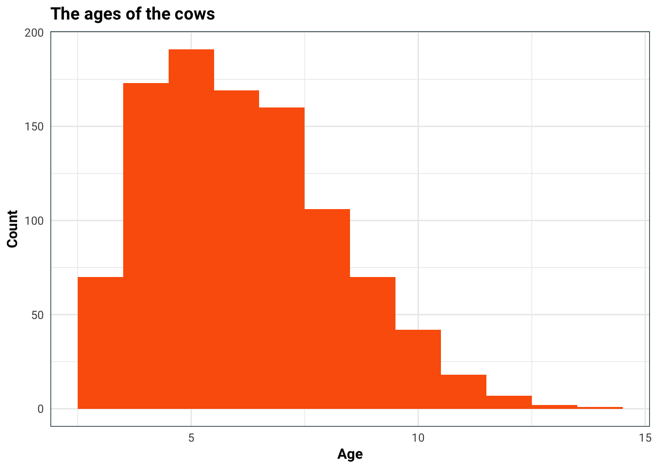
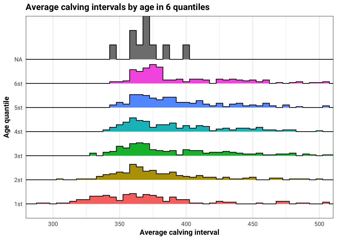
#> No. of test samples : 252We are trying to predict the average calving interval, so let us first take a look at it’s distribution. I am also concerned that age might be a factor in this, so I will split the histogram up.
library(ggridges)

training %>%
  ggplot(aes(Age)) +
  geom_histogram(binwidth = 1, fill = .colr[4]) +
  labs(
    title = "The ages of the cows",
    x = "Age",
    y = "Count"
  )
training %>%
  mutate(Age = ntile(Age, 6),
         Age = ifelse(!is.na(Age),
                      paste0(Age, "st"),
                      Age),
         Age = as.factor(Age)) %>%
  mutate(mean = mean(Average_calving_interval)) %>%
  ggplot(aes(Average_calving_interval, Age, fill = Age)) +
  geom_density_ridges(stat = "binline", binwidth = 5) +
  guides(fill = F) +
  coord_cartesian(xlim = c(290, 500)) +
  labs(
    title = "Average calving intervals by age in 6 quantiles",
    x = "Average calving interval",
    y = "Age quantile"
  )
Age does have quite an impact on average calving interval. This is most likely because for older cows, the average calving interval aggregates both their most fertile younger years, and the less fertile older years. This is something we should keep in mind when we build our model.
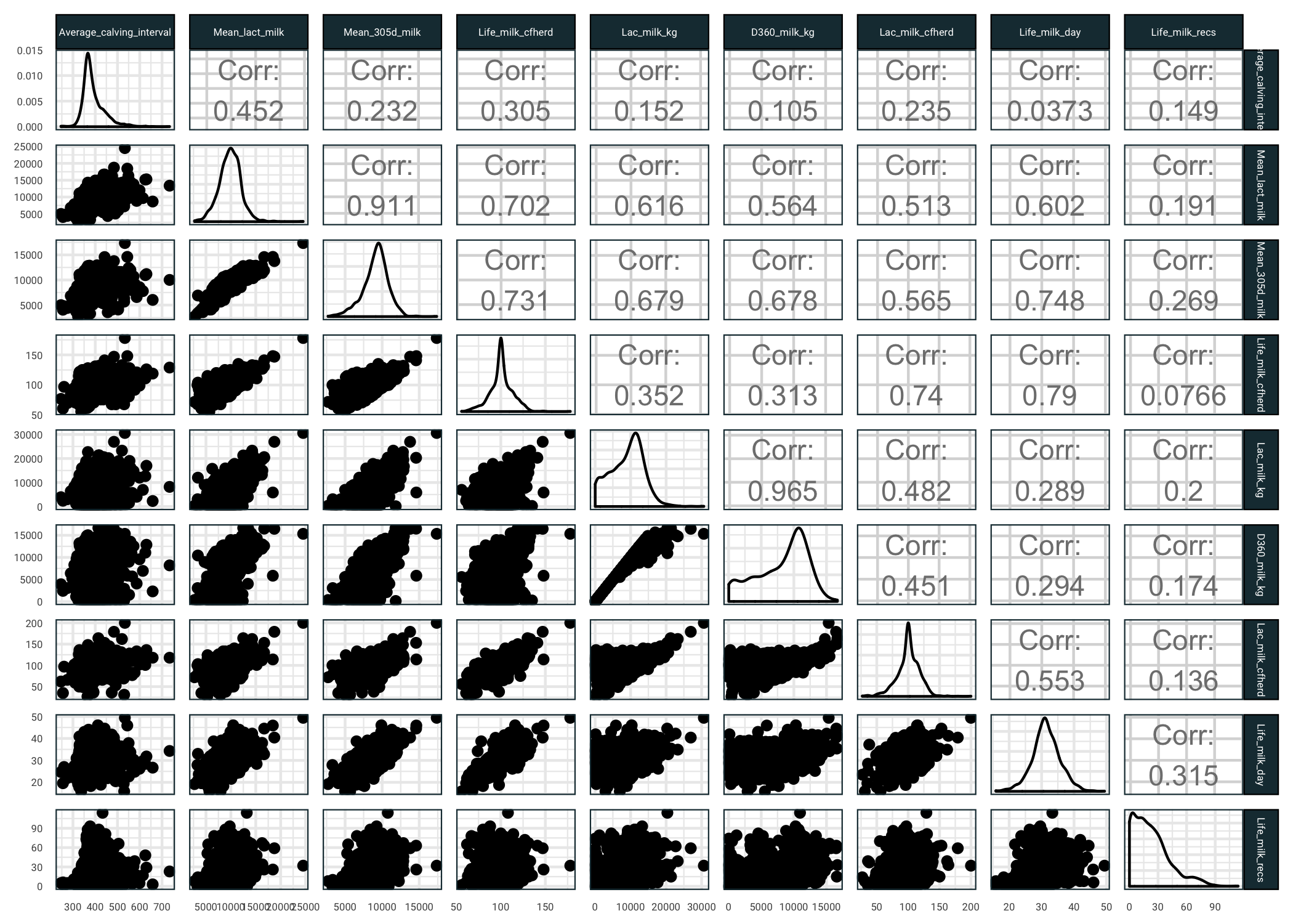
There are quite a few missing observations, which we will deal with later. For now our goal is to get an understanding of the predictors. Let us see some milk related predictors and how they relate to average calving interval (you might want to open the next image in a new tab).
library(GGally)
milk.ind = grep("*milk*", names(training))
milk.ind = c(which(names(training) == "Average_calving_interval"),
             milk.ind)
ggpairs(training[,milk.ind]) +
  theme(
    strip.text = element_text(size = 4),
    axis.text = element_text(size = 4)
  )
So several things we can see here:
- Average calving interval is pretty well correlated with mean lactose content of the cows milk
- The response has quite a high variance against the milk based predictors
- There are a few predictors that are highly correlated, we might want to remove some of these prior to fitting models
- Quite a few of the predictors have skewed distributions, we might want to use a transformation prior to fitting models
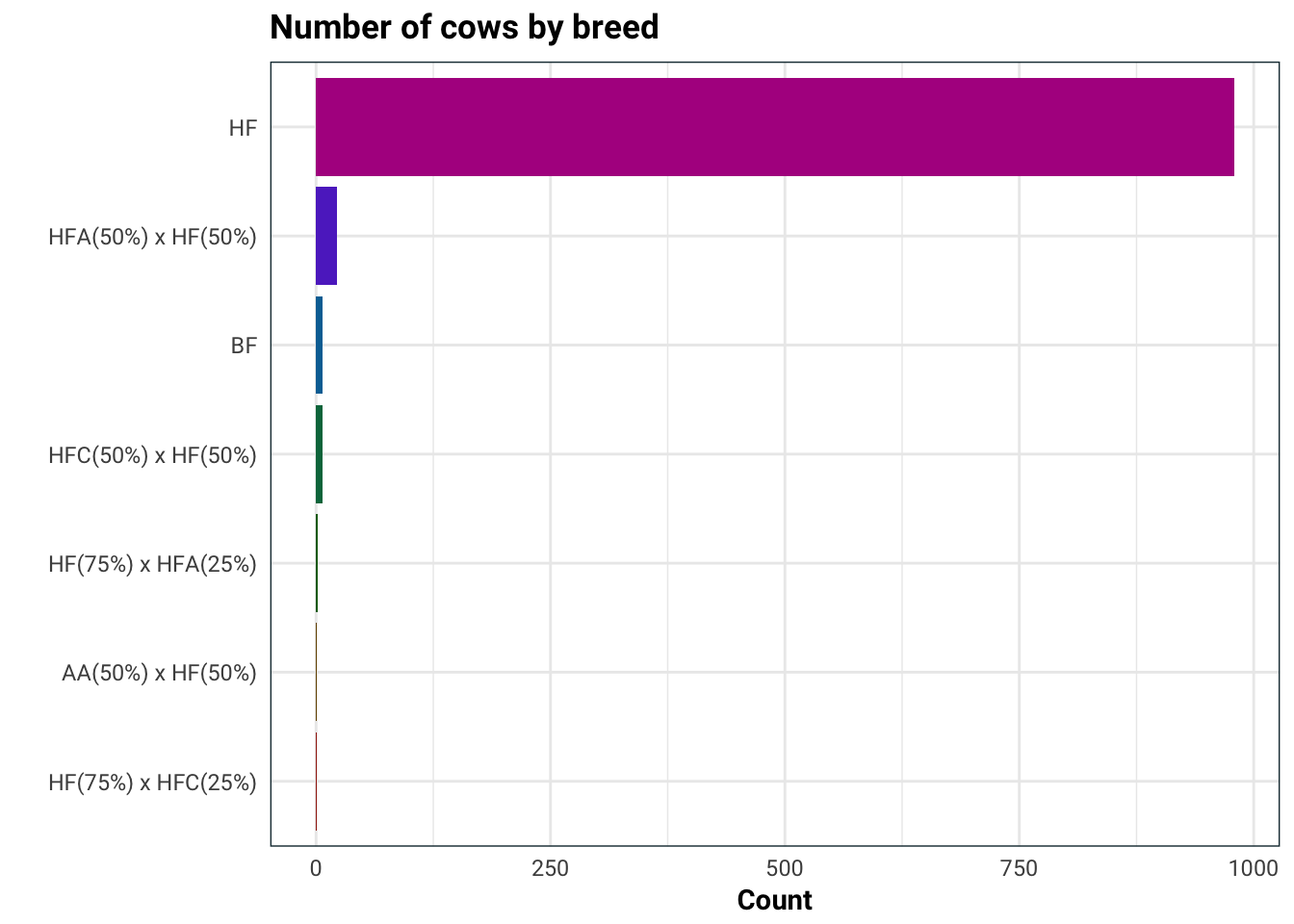
Next on the list is the breed of the cow.
library(forcats)
training %>%
  mutate(Breed = factor(Breed) %>%
           fct_infreq %>%
           fct_rev) %>%
  ggplot(aes(Breed, fill = Breed)) +
  geom_bar(stat = "count") +
  scale_fill_hue(l = 36) +
  guides(fill = F) +
  coord_flip() +
  labs(
    title = "Number of cows by breed",
    x = "",
    y = "Count"
  )
Seeing as the cows almost exclusively are of one breed, it would be best to not use this in our analysis.
That’s it for now, stay tuned for the second part where we will be setting up some juicy models to analyse this baby, or should I say calf.